I began backtesting three years ago and have executed over 25,000 backtests since then. I’ve taken several algo trading systems live intermittently. Bringing an immature backtested strategy to live trading can harm my capital, while bringing it to paper trading can be wasting time and computation power.
To mitigate these risks, I strive to validate backtest performance as thoroughly as possible before moving to paper or live trading.
The first step is reviewing the basics of backtest performance metrics. Building on this, I developed a Monte Carlo Simulation and Outlier Removal Validation Tool (details here).
In the age of AI, why not leverage AI to validate performance as well?
Steps Outline
Data Preparation
Performance Testing
Statistical Testing
Risk Assessment
Rating & Recommendation
(Remark - The prompts mentioned in this post tested in Gemini 3 Pro.)
Let’s start!
⚠️ IMPORTANT - This analysis validates the historical performance of completed trades and portfolio NAV. AI cannot validate if your backtest has: ❌ Overfitting ❌ Slipping & transaction cost harm the profit ❌ Look-ahead bias and survivorship bias ❌ Poor data quality ❌ Backtest program bug, etc
These problems can cause you to fail in real trading, even if your backtest performance is excellent!
Phase 1. Data Preparation
Prepare the data in the follow format
File 1 - Strategy & Benchmark (S&P500) Daily NAV in excel or csv format
Column 1 - Timestamp
Column 2 - Benchmark Daily NAV
Column 3 - Strategy daily NAV
e.g.
timestamp,benchmark value,strategy value
2020-01-02T21:00:00Z,100000.0,100503.7398
2020-01-03T21:00:00Z,99242.774,99584.3117
2020-01-06T21:00:00Z,99621.387,100225.1252
2020-01-07T21:00:00Z,99341.275,100211.1945
2020-01-08T21:00:00Z,99870.7175,100963.4538
2020-01-09T21:00:00Z,100547.9115,101817.8718
TASK 1: DATA PREPARATION

FILES PROVIDED:
- <NAV file name>: Daily strategy NAV and S&P500 benchmark values. Timestamp, Benchmark Daily NAV, Strategy daily NAV
- <trade file name>: Individual trade activity with Timestamp, Symbol, Price, Quantity

OUTPUT:
- Total Trading days
- Total Trades
- Date Ranges
- Assets Trade
- Data quality
- Any anomalies detected
LLM Response
The following report provides the data loading and validation results for the backtest analysis based on the provided files: Regime.xlsx (NAV data) and Regime Trade.xlsx (Trade activity).
…………. (removed due to limited text)
Phase 2. Performance Testing
2.1 - Portfolio Performance Metrics
LLM Prompt
TASK 2.1: PORTFOLIO PERFORMANCE METRICS

INSTRUCTIONS:

1. CALCULATE DAILY RETURNS
   - Strategy daily returns = (today_nav - yesterday_nav) / yesterday_nav × 100 (in %)
   - Benchmark daily returns = (today_sp500 - yesterday_sp500) / yesterday_sp500 × 100 (in %)

2. ANNUALIZED PERFORMANCE METRICS
   - Strategy Annual Return = (final_nav / initial_nav)^(252/trading_days) - 1
   - Benchmark Annual Return = (final_sp500 / initial_sp500)^(252/trading_days) - 1
   - Excess Annual Return (Alpha) = Strategy Annual Return - Benchmark Annual Return

3. RISK METRICS
   - Strategy Annual Volatility = Std Dev(daily returns) × √252
   - Benchmark Annual Volatility = Std Dev(daily returns) × √252
   - Correlation = Pearson correlation of strategy and benchmark daily returns


4. RISK-ADJUSTED RETURNS
   - Sharpe Ratio (Strategy) = (Strategy Annual Return - 0%) / Strategy Volatility
   - Sharpe Ratio (Benchmark) = (Benchmark Annual Return - 0%) / Benchmark Volatility
   - Calmar Ratio (Strategy) = Annual Return / Maximum Drawdown
   - Sortino Ratio (Strategy) = Annual Return / Downside Deviation (only negative returns)


5. MAXIMUM DRAWDOWN ANALYSIS
   - Cumulative NAV = Running product of (1 + daily_returns)
   - Running Maximum = Running max of cumulative NAV (high water mark)
   - Drawdown = (Running Max - Current Value) / Running Max × 100
   - Maximum Drawdown = Minimum drawdown value
   - Duration of Max Drawdown = Days from peak to recovery

6. MONTHLY & QUARTERLY AGGREGATION
   - Create monthly summary: Date, Return %, Win/Loss indicator
   - Create quarterly summary: Date, Return %, Win/Loss indicator
   - Calculate win rate: % of profitable months/quarters
   - Distribution analysis: 25th, 50th, 75th percentiles


7. SUMMARY
   - Provide a brief summary on the Strategy against Benchmark performances calculated above
   - Provide insights on the performance finding
LLM Response
Performance Analysis Summary
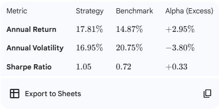
The following performance summary compares the Strategy against the Benchmark (S&P 500) from 2020-01-02 to 2025-12-31.
1. Annualized Performance Metrics
…………. (removed due to limited text)
Insights & Performance Findings
Superior Risk-Adjusted Returns: The strategy not only outperformed the benchmark by 2.95% annually but did so with significantly lower volatility 16.95% vs 20.75%. This resulted in a Sharpe Ratio 1.05 that is roughly 46% higher than the benchmark 0.72.
…………. (removed due to limited text)
2.2 - Trade Level Performance Metrics
LLM Prompt
TASK 2.3: TRADE LEVEL PERFORMANCE METRICS

INSTRUCTIONS:

1. CLASSIFY TRADES BY TRANSACTION TYPE
   - Entry Trade: Positive quantity (buying)
   - Exit Trade: Negative quantity (selling)

2. CREATE MATCHED PAIRS (For each symbol)
   - Match buy trades with subsequent sell trades (chronological order)
   - Calculate holding period in days: Exit_Date - Entry_Date
   - Calculate realized P&L: (Exit_Price × |Exit_Qty|) - (Entry_Price × Entry_Qty)
   - Calculate return %: Realized_PnL / (Entry_Price × Entry_Qty) × 100
   - Classify outcome: Win (>0% return) or Loss (≤0% return)

3. OVERALL TRADE STATISTICS
   For each asset:
   - Total completed trades (paired entries & exits)
   - Total trades executed (individual fills, including partial positions)
   - Average holding period (days)
   - Average trade return (%)
   - Percentage of winning trades
   - Percentage of losing trades
   - Average win size (%)
   - Average loss size (%)
   - Largest winning trade (%)
   - Largest losing trade (%)

4. PROFIT FACTOR CALCULATION
   - Gross Profit = Sum of all positive trade returns
   - Gross Loss = Sum of all negative trade returns (absolute value)
   - Profit Factor = Gross Profit / Gross Loss

5. CREATE TRADE ACTIVITY TABLE BY ASSET
   - including the following fields
      - asset
      - count
      - win rate
      - avg holding days
      - avg return
      - profit factor

6. SUMMARY
   - Provide insights on trade performance metrics
LLM Response
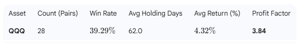
1. Trade Activity Summary
This table provides a high-level view of the strategy’s trading efficiency and performance per asset.
…………. (removed due to limited text)
Insights and Performance Findings
Positive Expectancy with Low Win Rate: The strategy demonstrates a “Fat Tail” or “Trend Following” characteristic. Despite losing more often than winning (60% loss rate), it remains highly profitable because the average win 14.87% is nearly 6 times larger than the average loss -2.51%.
…………. (removed due to limited text)
2.3 - Return Attribution Analysis
(Remark - LLM Response will be skipped from now on due to limited length limit)
TASK 2.3: RETURN ATTRIBUTION ANALYSIS

INSTRUCTIONS:

1. PERIOD DECOMPOSITION
   Divide backtest into 5-7 chronological periods (2-3 years each):

   For each period, calculate:
   - Period start/end dates
   - Strategy return (%)
   - Benchmark return (%)
   - Outperformance (%)
   - Dominant market regime (bull/bear/volatile)
   - Leading asset contributor

2. PERFORMANCE CONSISTENCY
   - Count periods where strategy outperformed benchmark
   - Period consistency = Outperform_Count / Total_Periods × 100%
   - Calculate rolling 12-month excess returns
   - Count months where rolling 12m strategy > benchmark
   - Rolling consistency = Outperform_Months / Total_Months × 100%

3. SUMMARY
   - Provide insights on return attribution analysis
2.4 - Regime Analysis
TASK 2.4: REGIME ANALYSIS

INSTRUCTIONS:

1. CLASSIFY MARKET REGIMES
   Using 60-day rolling window on benchmark:

   Calculate:
   - Rolling_60d_Return = % change over prior 60 days
   - Rolling_60d_Volatility = Std(daily returns, 60 days) × √252

   Regime definitions:
   - Bull/Low Vol: 60d_Return > 0 AND Volatility < 10%
   - Bull/High Vol: 60d_Return > 0 AND Volatility ≥ 10%
   - Bear/Low Vol: 60d_Return ≤ 0 AND Volatility < 10%
   - Bear/High Vol: 60d_Return ≤ 0 AND Volatility ≥ 10%
   - Crisis: Single-day benchmark drop > 3% (override other classifications)

2. REGIME PERFORMANCE STATISTICS
   For each regime, calculate:

┌──────────────────┬───────┬─────────────┬─────────────┬────────────┐
│ Regime           │ Days  │ Strat Avg   │ Bench Avg   │ Excess Ret │
│                  │       │ Daily Ret % │ Daily Ret % │    %       │
├──────────────────┼───────┼─────────────┼─────────────┼────────────┤
│ Bull/Low Vol     │  ___  │    ___%     │    ___%     │   ___%     │
│ Bull/High Vol    │  ___  │    ___%     │    ___%     │   ___%     │
│ Bear/Low Vol     │  ___  │    ___%     │    ___%     │   ___%     │
│ Bear/High Vol    │  ___  │    ___%     │    ___%     │   ___%     │
│ Crisis           │  ___  │    ___%     │    ___%     │   ___%     │
└──────────────────┴───────┴─────────────┴─────────────┴────────────┘

   Additionally for each regime:
   - Daily volatility (annualized)
   - Sharpe ratio (within regime)
   - Win rate (% positive days)
   - Max drawdown (during regime)

3. CRISIS PERIOD DEEP DIVE
   Identify 2-3 major crisis periods in backtest:

   For each crisis:
   - Peak NAV (pre-crisis)
   - Trough NAV
   - Maximum drawdown (%)
   - Strategy vs Benchmark drawdown
   - Outperformance during crisis
   - Days to 50% recovery
   - Days to full recovery

4. REGIME CONSISTENCY SCORE
   - Count regimes where strategy shows positive excess return
   - Consistency = Regimes_With_Outperformance / Total_Regimes

   Classification:
   - 80-100% (4-5 regimes): ✓ ROBUST
   - 50-79% (2-3 regimes): ⚠ REGIME-DEPENDENT
   - 0-49% (0-1 regimes): ✗ WEAK

5. SUMMARY
   - Provide insights on crisis analysis, regime performance & consistency
🚨 DO NOT PAPER TRADE YOUR ALGO BEFORE RUNNING ALL AI PROMPTS
Otherwise, you are wasting time to do it in paper trade. After 3-6 months, you find out the strategy is not going to work, you refine the backtest, and potentially wasting another 3-6 months!!!
Paid content to unlock the rest of testings
Statistical Testing - A scientific way to validate if your are not winning by luck!
Risk Assessment - Assessment to avoid losing everything overnight!
Rating & Recommendation ⭐⭐⭐ - Do you want to know if your strategy is A or not? AI also provides recommendation on your strategy!
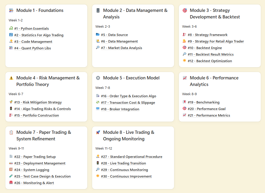
BONUS For Paid Member ONLY - “Champion’s Fast Lane Playbook: Master Algo Trading in 12 Weeks” - My 8 modules self-study guides and notes for building a winning strategy.